
|
|
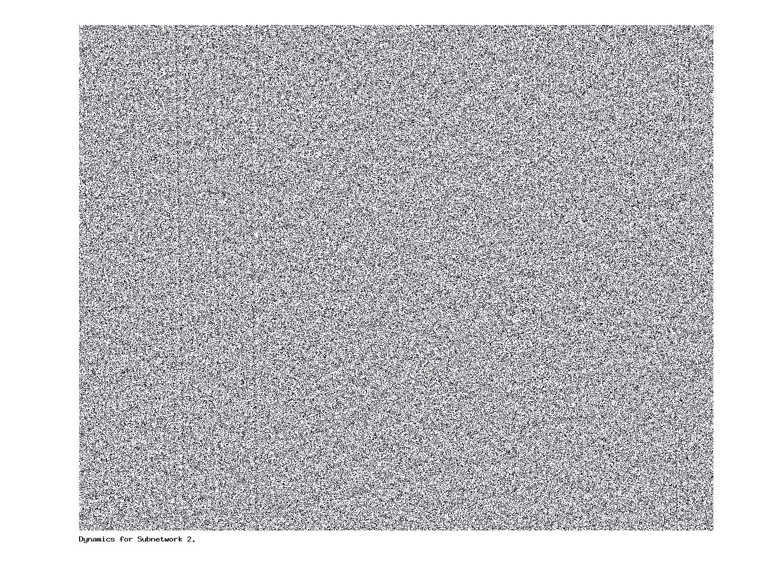
We show an example of adaptativity based on STDP. We assume we are given two networks \(\mathcal{N}_1\), \(\mathcal{N}_2\) each consisting of 400 weakly all-to-all coupled Kuramoto phase oscillators. The phase space of each oscillator is \([0,1]\) (mod 1). For \(\mathcal{N}_1\) we assume frequencies of the uncoupled oscillators are uniformly distributed in the interval [1.975,2.025] and that coupling is sufficient to ensure frequency synchonization and phase synchronization to within about \( \pm 7.5\%\). See figure 1 where we have plotted the dynamics of all 400 oscillators over a time period of approximately 2.5 seconds (discretized with a time step of 0.001).
|
|
Figure 2. Dynamics for \(\mathcal{N}_2\)
We assume cells in \(\mathcal{N}_1\), \(\mathcal{N}_2\) spike whenever the phase passes through one. We take a single target cell with a Leaky Integrate and Fire (LIF) dynamics, assume all 800 cells are connected to the target and that connection strengths (weights) are randomly assigned in the interval [0.1,1.8]. We assume weights are constrained to lie in [0,2]. For the simulation we show below we assume STDP which has multiplicative LTD and a power law LTP (exponent 0.5). We also assume a montone phase response curve for the target as well as a refractory period (for this simulation, the refractory period was 50ms).
|
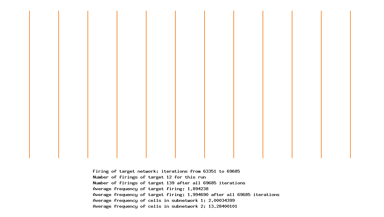
Figure 3. Firings of target cell after about 70 seconds of simulation.
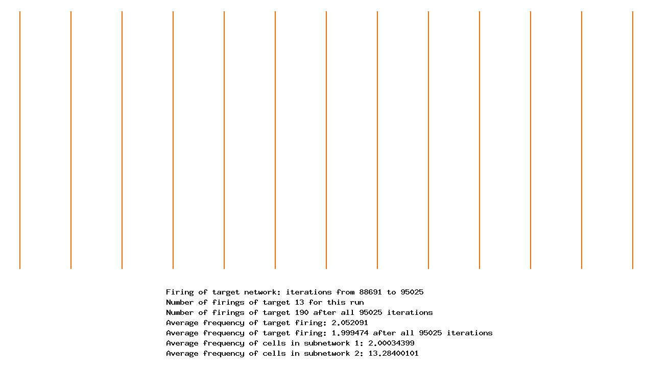
In figure 3 above, we show the firings of the target cell over a period of about 6 seconds. Over the whole simulation (run here for about 70 seconds of real time), the average frequency of firing of the target was 1.994690 compared with the average frequency of the cells in \(\mathcal{N}_1\) of 2.000343 - a difference of about 0.25%. Longer runs tend to give much closer approximations. We give the results of another simulation below in figure 4 where the difference is about 0.04% and the simulation was run about 95 seconds.
|
Figure 4. Firings of target cell after about 95 seconds of simulation.
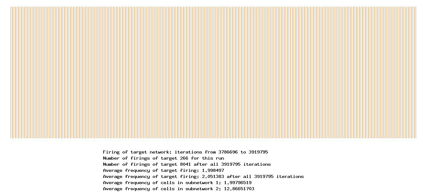
It typically takes anywhere from 30 to 60 seconds for the target cell dynamics to approximate those of \(\mathcal{N}_1\). The simulations above where done after this transient period. In some cases the weights of connections from \(\mathcal{N}_2\) to the target cell may all converge to zero; in other cases this does not happen. Nor do the weights from \(\mathcal{N}_1\) to the target necessarily go to an equilibrium state. In figure 5, we show the results of a simulation of about 2000 seconds for networks of size 100 and 50 respectively.
|
Figure 5. Firings of target cell after about 2000 seconds of simulation.
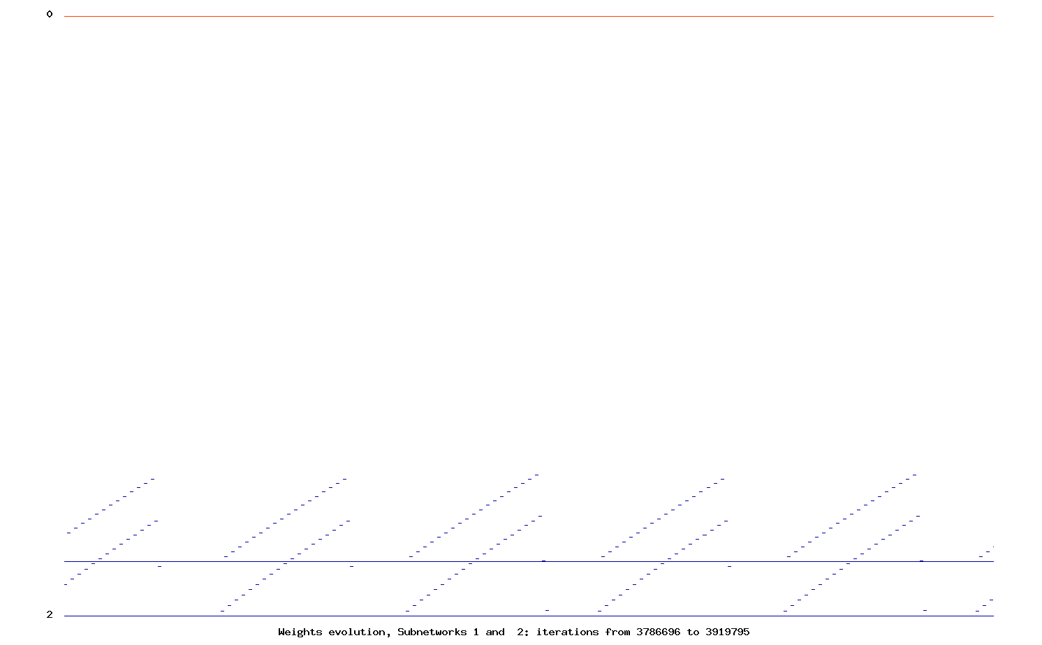
In this example, the connections from the second network all go to zero. On the other hand, the connections from the first network to the target cell do not converge to an equilibrium. See figure 6.
|
Figure 6. Weigths from \(\mathcal{N}_1\) to target cell
In figure 7, we show the average weight evolution (blue for \(\mathcal{N}_1\), orange for \(\mathcal{N}_2\)). Note that the curve for \(\mathcal{N}_1\) is not constant.

|
Figure 7. Average of weights from \(\mathcal{N}_1,\; \mathcal{N}_2\) to target cell
Research supported by NSF Grants DMS-1265253 and in collaboration with Anushaya Mohapatar (UH and Rice).
- Return to Mike Field's home page.
- DynamIC - Dynamical Systems, Imperial
- Imperial College Mathematics Department Home Page
- Rice University Mathematics Department Home Page
