Wavelet Spectrum Test
Description. This test of stationarity looks at a quantity called βj(t) which is closely related to a wavelet-based time-varying spectrum of the time series (it is a linear transform of the evolutionary wavelet spectrum of the locally stationary wavelet processes of Nason, von Sachs and Kroisandt, 2000). Again, we need to see whether the βj(t) function varies over time or is constant. Naturally, though, since we have data we need to examine an estimate of βj(t).
To verify constancy of βj(t) we use the technique due to von Sachs and Neumann (2000) which examines the Haar wavelet coefficients of the estimate of βj(t). A function f(t) is constant if and only if all of its Haar wavelet coefficients are zero. So, von Sachs and Neumann (2000) perform a multiple hypothesis test on all the Haar wavelet coefficients (of a potentially time-varying quantity) and is they are all deemed to be zero then the function is deemed to be constant. Von Sachs and Neumann (2000) develop powerful theory that establishes the asymptotic normality of the Haar wavelet coefficients under mild assumptions and for some time series with heavy tails also. Von Sachs and Neumann (2000) introduce this idea for local Fourier spectra and Nason (2013) applies it to wavelet spectra.
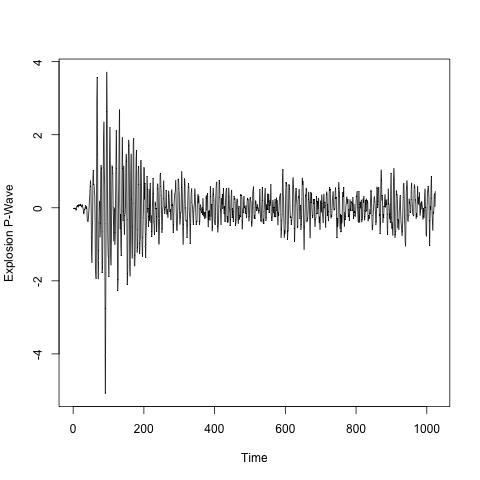
Implementation and Example. This test of stationarity can be found in the locits package as the hwtos2 function. We will continue our example from above and apply the test to the exP data set.
First, load the locits package, then apply the hwtos2 test and print out the results:
library("locits")
ans <- hwtos2(exP)
ans
The results are:
Class 'tos' : Stationarity Object :
~~~~ : List with 9 components with names
nreject rejpval spvals sTS AllTS AllPVal alpha x xSD
summary(.):
----------
There are 441 hypothesis tests altogether
There were 11 FDR rejects
The rejection p-value was 0.0002681456
Using Bonferroni rejection p-value is 0.0001133787
And there would be 9 rejections.
Listing FDR rejects... (thanks Y&Y!)
P: 7 HWTlev: 0 indices on next line...[1] 1
P: 7 HWTlev: 1 indices on next line...[1] 1
P: 7 HWTlev: 2 indices on next line...[1] 1
P: 7 HWTlev: 4 indices on next line...[1] 2
P: 7 HWTlev: 5 indices on next line...[1] 3
P: 8 HWTlev: 0 indices on next line...[1] 1
P: 8 HWTlev: 1 indices on next line...[1] 1
P: 8 HWTlev: 4 indices on next line...[1] 2
P: 9 HWTlev: 0 indices on next line...[1] 1
P: 9 HWTlev: 1 indices on next line...[1] 1
P: 9 HWTlev: 4 indices on next line...[1] 2
As mentioned above the test performs a multiple hypothesis test. There are various ways to assess the significance of multiple hypothesis tests and the output above shows assessment via Bonferroni correction and false discovery rate (FDR). It indicates that 11 hypothesis were rejected against FDR assessment and 9 according to Bonferroni. In either case the composite null hypothesis of stationarity is rejected and multiple null hypotheses are rejected. Wavelet Test of Stationarity
|